Tutorial 1. Getting started with RASP

Summary: An introductory tutorial to getting started with RASP. This tutorial describes the use of RASP to analyze Hawaiian Psychotria (Nepokroeff et al., 2003) data and infer biogeographic history using phylogenetic trees. It will take you through the process of importing trees, making choices about the model and generating a RASP result file.

This tutorial will guide you through running RASP to do a simple analysis. If you haven’t already, download and install RASP from:

http://mnh.scu.edu.cn/soft/blog/RASP (Binary)

https://sourceforge.net/projects/rasp2/files/ (Binary)

or https://github.com/sculab/RASP (source code)

The tutorials and example data could be downloaded from:

https://sourceforge.net/projects/rasp2/files/Tutorials.zip

or http://mnh.scu.edu.cn/soft/blog/RASP/Tutorials.zip

Running RASP for the first time

For MacOS users, please move RASP.app into the Application folder to avoid compatibility issues. For Windows users, we strongly recommend showing the extension of files. Run RASP by double clicking on its icon. Once running, RASP will look similar irrespective of which computer system it is running on. For this tutorial, the Windows version will be shown but the MacOS versions will have exactly the same layout and functionality.

Loading the tree files

When running, you will see a window like this:

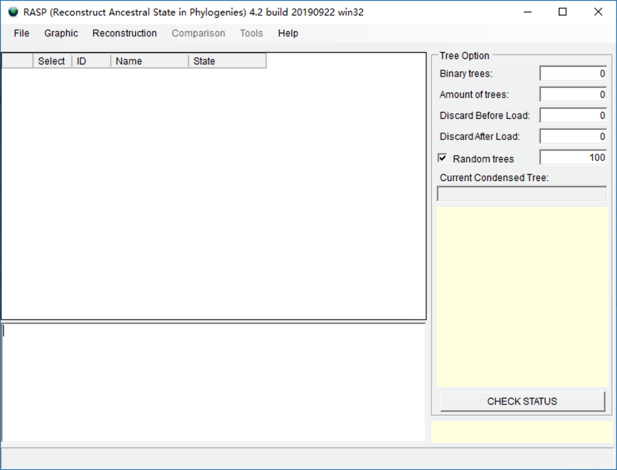
The first thing you need to do is to load a consensus tree or trees dataset. Trees can be obtained from common phylogenetic packages such as BEAST, MEGA, MrBayes, TNT and many others. In this tutorial, all files are stored in examples/Psychotria/ folder.

The examples/Psychotria/Trees_States folder in the RASP download package contains a trees dataset called dataset.trees and a consensus tree called Psychotria.tree.

NOTE: The dataset.trees, which contains 1001 posterior trees, is generated in BEAST using the fasta files in the examples/Psychotria/Alignments folder. The Psychotria.tree is the maximum clade credibility (MCC) tree of dataset.trees obtained using the program TreeAnnotator in BEAST.

Open [File > Load Trees> Load Trees (more format)] and navigate to dataset.trees and select it.

Open [File> Load Consensus Tree> Load User-specified Tree] and navigate to Psychotria.tree and select it.

NOTE: If you have one tree only, you could load it using [File > Load Trees> Load Trees (more format)] and do not need to load it again using [File> Load Condensed Tree> Load User-specified Tree].

NOTE: If you want to look at the consensus tree, click [ Graphic > Tree View].

Loading the distribution file

You can input and revise the states (distributions) in the entry fields in the “State” column in RASP. Alternatively, users can load a states file that was previously generated. In this tutorial, we have already made a state file in

examples/Psychotria/Trees_States/distribution.csv

Open [File > Load States (Distributions)], navigate to distribution.csv and select it. Now you will see a window like this:

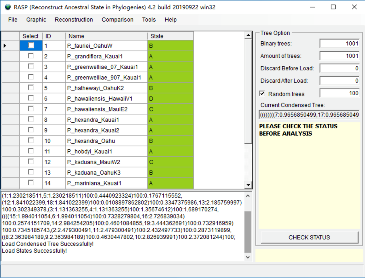
NOTE: Users can open and edit the distribution.csv file with Excel. The columns in distribution.csv are the ID, species names and distribution (state). The species names need to be exactly the same as those in the RASP window, but the order of species names does not.

NOTE: The A, B, C and D in the distribution.csv file indicate different distribution areas. If a species is distributed in both A and C, the distribution should be AC. RASP requires users to use continuous letters to represent distribution areas. For instance, if you have four areas, they should be A, B, C and D, but not A, C, D, E.

NOTE: We recommend users to click “CHECK STATUS” after any changes to their trees or distributions. It will show useful error and warning messages, and tell you which analyses can be done at the current status.

Running a classical S-DIVA model

For our first analysis we will run a Statistical Dispersal-Vicariance Analysis (S-DIVA) analysis to infer biogeographic history through multiple phylogenetic trees. Using multiple trees instead of one (e.g. consensus) tree allows users to explicitly accommodate phylogenetic uncertainty into models. Open [Reconstruction> On Trees> Statistical Dispersal-Vicariance Analysis (S-DIVA)], you will see a window like the following:

Users can keep everything as default and click OK (See 3.3.5 in Manual of RASP for the details of settings). You may see a command window (in Windows) with some text. Keep it open until it closes automatically. This analysis took 3 seconds to run on a 3.0 GHz CPU. The “Threads” option can be used to increase the speed of analyses that are more computationally intensive.

The most important parameter here is “Max areas at each node”. It defines the number of unit areas allowed in ancestral distributions. The list of “Include” will be updated when you change the value of “Max areas at each node”.

NOTE: The value of “Max areas at each node” can be set as the maximum number of unit areas of current species or even the total number of your areas. However, these settings may also lead to a wide distribution at the root node. Users can restrict this value to obtain a more meaningful result.

Visualizing the result

Open [Graphic->Tree View] and you will see a window like this:

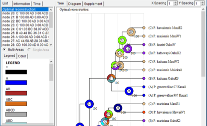
Open [File> Save Result] to save the result. Open [File> Export Graphic> Export Tree] and [File> Export Graphic> Export Legend] to save the tree and legend, respectively.

If you are using a dated tree, you could go to the “Time” tab and click “Calculate”. In the image below, the X-axis represents time and the Y-axis is the density of different events on the tree.

Open [File> Export Graphic> Export Diagram] to save the graphic.

NOTE: Double click on a node in the picture to select the node, and double click on any blank space to cancel node select. You can also select nodes using the list towards the left of the window.

NOTE: Typically, nodes from the tree are drawn in increasing node order (go to [View> Rearrange Tree] to do so). Users can also change the view of the tree using [View> Option].

NOTE: Users can export graphics to vectorial drawing (.svg/wmf file, compatible with Adobe Illustrator) or picture (.png file) format.

References:

Nepokroeff, M., Sytsma, K. J., Wagner, W. L., & Zimmer, E. A. (2003). Reconstructing Ancestral Patterns of Colonization and Dispersal in the Hawaiian Understory Tree Genus Psychotria (Rubiaceae); A Comparison of Parsimony and Likelihood Approaches. Systematic Biology, 52(6), 820-838